Before begin…
CS231n exercise1.2 : SVM에 대한 본인의 풀이이다. 자세한 코드는 github에서 확인 가능하다.
Multiclass Support Vector Machine exercise
Complete and hand in this completed worksheet (including its outputs and any supporting code outside of the worksheet) with your assignment submission. For more details see the assignments page on the course website.
In this exercise you will:
- implement a fully-vectorized loss function for the SVM
- implement the fully-vectorized expression for its analytic gradient
- check your implementation using numerical gradient
- use a validation set to tune the learning rate and regularization strength
- optimize the loss function with SGD
- visualize the final learned weights
1
2
3
4
5
6
7
8
9
10
11
12
13
14
15
16
17
| # Run some setup code for this notebook.
import random
import numpy as np
from cs231n.data_utils import load_CIFAR10
import matplotlib.pyplot as plt
# This is a bit of magic to make matplotlib figures appear inline in the
# notebook rather than in a new window.
%matplotlib inline
plt.rcParams['figure.figsize'] = (10.0, 8.0) # set default size of plots
plt.rcParams['image.interpolation'] = 'nearest'
plt.rcParams['image.cmap'] = 'gray'
# Some more magic so that the notebook will reload external python modules;
# see http://stackoverflow.com/questions/1907993/autoreload-of-modules-in-ipython
%load_ext autoreload
%autoreload 2
|
CIFAR-10 Data Loading and Preprocessing
1
2
3
4
5
6
7
8
9
10
11
12
13
14
15
16
17
18
| # Load the raw CIFAR-10 data.
cifar10_dir = 'cs231n/datasets/cifar-10-batches-py'
# Cleaning up variables to prevent loading data multiple times (which may cause memory issue)
try:
del X_train, y_train
del X_test, y_test
print('Clear previously loaded data.')
except:
pass
X_train, y_train, X_test, y_test = load_CIFAR10(cifar10_dir)
# As a sanity check, we print out the size of the training and test data.
print('Training data shape: ', X_train.shape)
print('Training labels shape: ', y_train.shape)
print('Test data shape: ', X_test.shape)
print('Test labels shape: ', y_test.shape)
|
1
2
3
4
| Training data shape: (50000, 32, 32, 3)
Training labels shape: (50000,)
Test data shape: (10000, 32, 32, 3)
Test labels shape: (10000,)
|
1
2
3
4
5
6
7
8
9
10
11
12
13
14
15
16
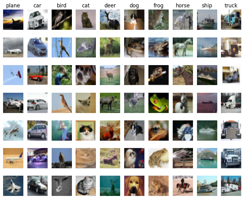
| # Visualize some examples from the dataset.
# We show a few examples of training images from each class.
classes = ['plane', 'car', 'bird', 'cat', 'deer', 'dog', 'frog', 'horse', 'ship', 'truck']
num_classes = len(classes)
samples_per_class = 7
for y, cls in enumerate(classes):
idxs = np.flatnonzero(y_train == y)
idxs = np.random.choice(idxs, samples_per_class, replace=False)
for i, idx in enumerate(idxs):
plt_idx = i * num_classes + y + 1
plt.subplot(samples_per_class, num_classes, plt_idx)
plt.imshow(X_train[idx].astype('uint8'))
plt.axis('off')
if i == 0:
plt.title(cls)
plt.show()
|
1
2
3
4
5
6
7
8
9
10
11
12
13
14
15
16
17
18
19
20
21
22
23
24
25
26
27
28
29
30
31
32
33
34
35
36
37
38
| # Split the data into train, val, and test sets. In addition we will
# create a small development set as a subset of the training data;
# we can use this for development so our code runs faster.
num_training = 49000
num_validation = 1000
num_test = 1000
num_dev = 500
# Our validation set will be num_validation points from the original
# training set.
mask = range(num_training, num_training + num_validation)
X_val = X_train[mask]
y_val = y_train[mask]
# Our training set will be the first num_train points from the original
# training set.
mask = range(num_training)
X_train = X_train[mask]
y_train = y_train[mask]
# We will also make a development set, which is a small subset of
# the training set.
mask = np.random.choice(num_training, num_dev, replace=False)
X_dev = X_train[mask]
y_dev = y_train[mask]
# We use the first num_test points of the original test set as our
# test set.
mask = range(num_test)
X_test = X_test[mask]
y_test = y_test[mask]
print('Train data shape: ', X_train.shape)
print('Train labels shape: ', y_train.shape)
print('Validation data shape: ', X_val.shape)
print('Validation labels shape: ', y_val.shape)
print('Test data shape: ', X_test.shape)
print('Test labels shape: ', y_test.shape)
|
1
2
3
4
5
6
| Train data shape: (49000, 32, 32, 3)
Train labels shape: (49000,)
Validation data shape: (1000, 32, 32, 3)
Validation labels shape: (1000,)
Test data shape: (1000, 32, 32, 3)
Test labels shape: (1000,)
|
1
2
3
4
5
6
7
8
9
10
11
| # Preprocessing: reshape the image data into rows
X_train = np.reshape(X_train, (X_train.shape[0], -1))
X_val = np.reshape(X_val, (X_val.shape[0], -1))
X_test = np.reshape(X_test, (X_test.shape[0], -1))
X_dev = np.reshape(X_dev, (X_dev.shape[0], -1))
# As a sanity check, print out the shapes of the data
print('Training data shape: ', X_train.shape)
print('Validation data shape: ', X_val.shape)
print('Test data shape: ', X_test.shape)
print('dev data shape: ', X_dev.shape)
|
1
2
3
4
| Training data shape: (49000, 3072)
Validation data shape: (1000, 3072)
Test data shape: (1000, 3072)
dev data shape: (500, 3072)
|
1
2
3
4
5
6
7
8
9
10
11
12
13
14
15
16
17
18
19
20
21
22
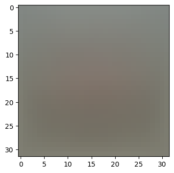
| # Preprocessing: subtract the mean image
# first: compute the image mean based on the training data
mean_image = np.mean(X_train, axis=0)
print(mean_image[:10]) # print a few of the elements
plt.figure(figsize=(4,4))
plt.imshow(mean_image.reshape((32,32,3)).astype('uint8')) # visualize the mean image
plt.show()
# second: subtract the mean image from train and test data
X_train -= mean_image
X_val -= mean_image
X_test -= mean_image
X_dev -= mean_image
# third: append the bias dimension of ones (i.e. bias trick) so that our SVM
# only has to worry about optimizing a single weight matrix W.
X_train = np.hstack([X_train, np.ones((X_train.shape[0], 1))])
X_val = np.hstack([X_val, np.ones((X_val.shape[0], 1))])
X_test = np.hstack([X_test, np.ones((X_test.shape[0], 1))])
X_dev = np.hstack([X_dev, np.ones((X_dev.shape[0], 1))])
print(X_train.shape, X_val.shape, X_test.shape, X_dev.shape)
|
1
2
| [130.64189796 135.98173469 132.47391837 130.05569388 135.34804082
131.75402041 130.96055102 136.14328571 132.47636735 131.48467347]
|
1
| (49000, 3073) (1000, 3073) (1000, 3073) (500, 3073)
|
SVM Classifier
Your code for this section will all be written inside cs231n/classifiers/linear_svm.py.
As you can see, we have prefilled the function svm_loss_naive which uses for loops to evaluate the multiclass SVM loss function.
\[\text{margin} = s_j-s_{y_i} + \delta\]
1
2
3
4
5
6
7
8
9
| # Evaluate the naive implementation of the loss we provided for you:
from cs231n.classifiers.linear_svm import svm_loss_naive
import time
# generate a random SVM weight matrix of small numbers
W = np.random.randn(3073, 10) * 0.0001
loss, grad = svm_loss_naive(W, X_dev, y_dev, 0.000005)
print('loss: %f' % (loss, ))
|
The grad returned from the function above is right now all zero. Derive and implement the gradient for the SVM cost function and implement it inline inside the function svm_loss_naive. You will find it helpful to interleave your new code inside the existing function.
To check that you have correctly implemented the gradient, you can numerically estimate the gradient of the loss function and compare the numeric estimate to the gradient that you computed. We have provided code that does this for you:
1
2
3
4
5
6
7
8
9
10
11
12
13
14
15
16
17
18
| # Once you've implemented the gradient, recompute it with the code below
# and gradient check it with the function we provided for you
# Compute the loss and its gradient at W.
loss, grad = svm_loss_naive(W, X_dev, y_dev, 0.0)
# Numerically compute the gradient along several randomly chosen dimensions, and
# compare them with your analytically computed gradient. The numbers should match
# almost exactly along all dimensions.
from cs231n.gradient_check import grad_check_sparse
f = lambda w: svm_loss_naive(w, X_dev, y_dev, 0.0)[0]
grad_numerical = grad_check_sparse(f, W, grad)
# do the gradient check once again with regularization turned on
# you didn't forget the regularization gradient did you?
loss, grad = svm_loss_naive(W, X_dev, y_dev, 5e1)
f = lambda w: svm_loss_naive(w, X_dev, y_dev, 5e1)[0]
grad_numerical = grad_check_sparse(f, W, grad)
|
1
2
3
4
5
6
7
8
9
10
11
12
13
14
15
16
17
18
19
20
| numerical: -36.292117 analytic: -36.292117, relative error: 1.297052e-11
numerical: 7.943945 analytic: 7.943945, relative error: 7.680180e-11
numerical: -19.932553 analytic: -19.932553, relative error: 2.671511e-11
numerical: 6.113729 analytic: 6.113729, relative error: 3.142132e-11
numerical: 14.408637 analytic: 14.408637, relative error: 2.021860e-14
numerical: 12.440661 analytic: 12.440661, relative error: 1.954039e-11
numerical: 19.977240 analytic: 19.977240, relative error: 8.951212e-12
numerical: 14.810861 analytic: 14.810861, relative error: 9.910440e-12
numerical: -25.557649 analytic: -25.557649, relative error: 6.744591e-12
numerical: 11.938094 analytic: 11.938094, relative error: 5.122498e-12
numerical: 2.564199 analytic: 2.564199, relative error: 1.760372e-11
numerical: -1.984778 analytic: -1.984778, relative error: 7.631527e-12
numerical: 29.909729 analytic: 29.909729, relative error: 1.782223e-11
numerical: 15.048738 analytic: 15.048738, relative error: 1.613970e-11
numerical: 23.186077 analytic: 23.186077, relative error: 1.203446e-11
numerical: 4.419457 analytic: 4.419457, relative error: 2.345793e-11
numerical: 27.798558 analytic: 27.798558, relative error: 6.669991e-13
numerical: -25.815624 analytic: -25.815624, relative error: 2.155509e-11
numerical: 13.017248 analytic: 13.017248, relative error: 4.785510e-12
numerical: 15.317591 analytic: 15.317591, relative error: 1.288972e-11
|
Inline Question 1
It is possible that once in a while a dimension in the gradcheck will not match exactly. What could such a discrepancy be caused by? Is it a reason for concern? What is a simple example in one dimension where a gradient check could fail? How would change the margin affect of the frequency of this happening? Hint: the SVM loss function is not strictly speaking differentiable
$\color{blue}{\textit Your Answer:}$
Gradient Checking? Numerical diffrerential과 역전파 계산한 analytic gradient를 비교하여 구현이 올바른지 검증하는 방법. 이 방식은 함수가 모든 지점에서 미분 가능할 때만 정확한 값을 찾을 수 있음.
\[\frac{\partial f}{\partial x} \approx \frac{f(x+h)-f(x-h}{2h}\]
SVM의 hinge loss 함수는 $max(0,x)$를 포함하므로 $x=0$에서 미분이 정의되지 않음
\[L_i = \sum_{j\ne y_i}\max(0,s_j-s_{y_i}+Δ)\]
종합하면
- SVM loss는 입력값이 $s_j-s_{y_i}+Δ=0$인 포인트 근처에 있을 경우 수치 미분이 일치하지 않을 수 있음
- 심각한 문제는 아니지만 오차가 일관되고 크면 구현 오류 가능성 상승
- 상술했듯이 $x=0$에서 미분 불가능
- 마진 $\delta$ 값을 크게 늘리면 더 많은 표본이 힌지 로스 함수에 걸리게 되무로 미분이 정의되지 않는 지점이 많아짐. 따라서 gradient check가 실패할 가능성이 높아지고 vice versa.
1
2
3
4
5
6
7
8
9
10
11
12
13
14
15
| # Next implement the function svm_loss_vectorized; for now only compute the loss;
# we will implement the gradient in a moment.
tic = time.time()
loss_naive, grad_naive = svm_loss_naive(W, X_dev, y_dev, 0.000005)
toc = time.time()
print('Naive loss: %e computed in %fs' % (loss_naive, toc - tic))
from cs231n.classifiers.linear_svm import svm_loss_vectorized
tic = time.time()
loss_vectorized, _ = svm_loss_vectorized(W, X_dev, y_dev, 0.000005)
toc = time.time()
print('Vectorized loss: %e computed in %fs' % (loss_vectorized, toc - tic))
# The losses should match but your vectorized implementation should be much faster.
print('difference: %f' % (loss_naive - loss_vectorized))
|
1
2
3
| Naive loss: 9.025805e+00 computed in 0.045247s
Vectorized loss: 9.025805e+00 computed in 0.011504s
difference: 0.000000
|
1
2
3
4
5
6
7
8
9
10
11
12
13
14
15
16
17
18
19
20
| # Complete the implementation of svm_loss_vectorized, and compute the gradient
# of the loss function in a vectorized way.
# The naive implementation and the vectorized implementation should match, but
# the vectorized version should still be much faster.
tic = time.time()
_, grad_naive = svm_loss_naive(W, X_dev, y_dev, 0.000005)
toc = time.time()
print('Naive loss and gradient: computed in %fs' % (toc - tic))
tic = time.time()
_, grad_vectorized = svm_loss_vectorized(W, X_dev, y_dev, 0.000005)
toc = time.time()
print('Vectorized loss and gradient: computed in %fs' % (toc - tic))
# The loss is a single number, so it is easy to compare the values computed
# by the two implementations. The gradient on the other hand is a matrix, so
# we use the Frobenius norm to compare them.
difference = np.linalg.norm(grad_naive - grad_vectorized, ord='fro')
print('difference: %f' % difference)
|
1
2
3
| Naive loss and gradient: computed in 0.044702s
Vectorized loss and gradient: computed in 0.010179s
difference: 0.000000
|
Stochastic Gradient Descent
We now have vectorized and efficient expressions for the loss, the gradient and our gradient matches the numerical gradient. We are therefore ready to do SGD to minimize the loss. Your code for this part will be written inside cs231n/classifiers/linear_classifier.py.
1
2
3
4
5
6
7
8
9
| # In the file linear_classifier.py, implement SGD in the function
# LinearClassifier.train() and then run it with the code below.
from cs231n.classifiers import LinearSVM
svm = LinearSVM()
tic = time.time()
loss_hist = svm.train(X_train, y_train, learning_rate=1e-7, reg=2.5e4,
num_iters=1500, verbose=True)
toc = time.time()
print('That took %fs' % (toc - tic))
|
1
2
3
4
5
6
7
8
9
10
11
12
13
14
15
16
| iteration 0 / 1500: loss 792.462188
iteration 100 / 1500: loss 287.882125
iteration 200 / 1500: loss 108.275734
iteration 300 / 1500: loss 42.543002
iteration 400 / 1500: loss 18.790975
iteration 500 / 1500: loss 10.428685
iteration 600 / 1500: loss 7.067637
iteration 700 / 1500: loss 6.056839
iteration 800 / 1500: loss 5.041565
iteration 900 / 1500: loss 5.522890
iteration 1000 / 1500: loss 5.026256
iteration 1100 / 1500: loss 5.669200
iteration 1200 / 1500: loss 5.354353
iteration 1300 / 1500: loss 5.160691
iteration 1400 / 1500: loss 5.656526
That took 12.223492s
|
1
2
3
4
5
6
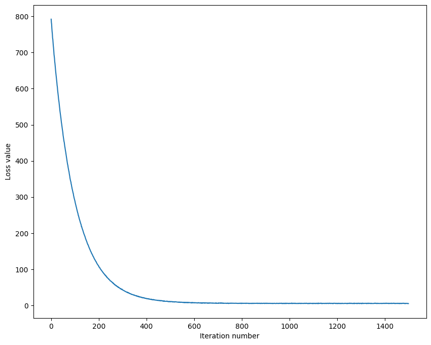
| # A useful debugging strategy is to plot the loss as a function of
# iteration number:
plt.plot(loss_hist)
plt.xlabel('Iteration number')
plt.ylabel('Loss value')
plt.show()
|
1
2
3
4
5
6
| # Write the LinearSVM.predict function and evaluate the performance on both the
# training and validation set
y_train_pred = svm.predict(X_train)
print('training accuracy: %f' % (np.mean(y_train == y_train_pred), ))
y_val_pred = svm.predict(X_val)
print('validation accuracy: %f' % (np.mean(y_val == y_val_pred), ))
|
1
2
| training accuracy: 0.364714
validation accuracy: 0.370000
|
1
2
3
4
5
6
7
8
9
10
11
12
13
14
15
16
17
18
19
20
21
22
23
24
25
26
27
28
29
30
31
32
33
34
35
36
37
38
39
40
41
42
43
44
45
46
47
48
49
50
51
52
53
54
55
56
57
58
59
60
61
62
63
64
65
66
67
68
69
| # Use the validation set to tune hyperparameters (regularization strength and
# learning rate). You should experiment with different ranges for the learning
# rates and regularization strengths; if you are careful you should be able to
# get a classification accuracy of about 0.39 (> 0.385) on the validation set.
# Note: you may see runtime/overflow warnings during hyper-parameter search.
# This may be caused by extreme values, and is not a bug.
# results is dictionary mapping tuples of the form
# (learning_rate, regularization_strength) to tuples of the form
# (training_accuracy, validation_accuracy). The accuracy is simply the fraction
# of data points that are correctly classified.
results = {}
best_val = -1 # The highest validation accuracy that we have seen so far.
best_svm = None # The LinearSVM object that achieved the highest validation rate.
################################################################################
# TODO: #
# Write code that chooses the best hyperparameters by tuning on the validation #
# set. For each combination of hyperparameters, train a linear SVM on the #
# training set, compute its accuracy on the training and validation sets, and #
# store these numbers in the results dictionary. In addition, store the best #
# validation accuracy in best_val and the LinearSVM object that achieves this #
# accuracy in best_svm. #
# #
# Hint: You should use a small value for num_iters as you develop your #
# validation code so that the SVMs don't take much time to train; once you are #
# confident that your validation code works, you should rerun the validation #
# code with a larger value for num_iters. #
################################################################################
# Provided as a reference. You may or may not want to change these hyperparameters
# 확인할 하이퍼 파라미터들 추가
learning_rates = [1e-7, 5e-5,3,5]
regularization_strengths = [2.5e4, 5e4,3,5]
iterations = [50, 100]
batch_size = [100,200,300]
# *****START OF YOUR CODE (DO NOT DELETE/MODIFY THIS LINE)*****
import itertools # for문 네 개 쓰는것보다 itertools 쓰는게 더 직관적
for lr, reg, iters, batch in itertools.product(
learning_rates, regularization_strengths,iterations, batch_size
):
svm = LinearSVM() # 모델 객체 생성
svm.train(
X_train, y_train, learning_rate=lr, reg=reg, num_iters=iters, batch_size=batch
) # 훈련
y_train_pred = svm.predict(X_train)
y_val_pred = svm.predict(X_val)
train_acc = np.mean(y_train == y_train_pred)
val_acc = np.mean(y_val == y_val_pred)
results[(lr,reg)] = (train_acc, val_acc)
if best_val < val_acc:
best_val = val_acc
best_svm = svm
# *****END OF YOUR CODE (DO NOT DELETE/MODIFY THIS LINE)*****
# Print out results.
for lr, reg in sorted(results):
train_accuracy, val_accuracy = results[(lr, reg)]
print('lr %e reg %e train accuracy: %f val accuracy: %f' % (
lr, reg, train_accuracy, val_accuracy))
print('best validation accuracy achieved during cross-validation: %f' % best_val)
|
1
2
3
4
5
6
7
8
9
10
11
12
13
14
15
16
17
18
19
20
21
22
23
24
25
26
27
28
29
30
31
32
33
34
35
| /usr/local/lib/python3.11/dist-packages/numpy/_core/fromnumeric.py:86: RuntimeWarning: overflow encountered in reduce
return ufunc.reduce(obj, axis, dtype, out, **passkwargs)
/content/drive/My Drive/cs231n/assignments/assignment1/cs231n/classifiers/linear_svm.py:96: RuntimeWarning: overflow encountered in multiply
loss += reg * np.sum(W*W)
/content/drive/My Drive/cs231n/assignments/assignment1/cs231n/classifiers/linear_svm.py:119: RuntimeWarning: overflow encountered in multiply
dW += 2 * reg * W
/content/drive/My Drive/cs231n/assignments/assignment1/cs231n/classifiers/linear_classifier.py:88: RuntimeWarning: overflow encountered in multiply
self.W -= learning_rate * grad # Vanilla Gradient Descent 응용 step size == learning rate
/content/drive/My Drive/cs231n/assignments/assignment1/cs231n/classifiers/linear_classifier.py:88: RuntimeWarning: invalid value encountered in subtract
self.W -= learning_rate * grad # Vanilla Gradient Descent 응용 step size == learning rate
/content/drive/My Drive/cs231n/assignments/assignment1/cs231n/classifiers/linear_svm.py:96: RuntimeWarning: overflow encountered in scalar multiply
loss += reg * np.sum(W*W)
/content/drive/My Drive/cs231n/assignments/assignment1/cs231n/classifiers/linear_svm.py:92: RuntimeWarning: overflow encountered in subtract
margins = np.maximum(0, scores-correct_scores + 1)
/content/drive/My Drive/cs231n/assignments/assignment1/cs231n/classifiers/linear_svm.py:92: RuntimeWarning: invalid value encountered in subtract
margins = np.maximum(0, scores-correct_scores + 1)
lr 1.000000e-07 reg 3.000000e+00 train accuracy: 0.204694 val accuracy: 0.228000
lr 1.000000e-07 reg 5.000000e+00 train accuracy: 0.211918 val accuracy: 0.227000
lr 1.000000e-07 reg 2.500000e+04 train accuracy: 0.219327 val accuracy: 0.233000
lr 1.000000e-07 reg 5.000000e+04 train accuracy: 0.244939 val accuracy: 0.257000
lr 5.000000e-05 reg 3.000000e+00 train accuracy: 0.260531 val accuracy: 0.248000
lr 5.000000e-05 reg 5.000000e+00 train accuracy: 0.246571 val accuracy: 0.251000
lr 5.000000e-05 reg 2.500000e+04 train accuracy: 0.064061 val accuracy: 0.072000
lr 5.000000e-05 reg 5.000000e+04 train accuracy: 0.048245 val accuracy: 0.050000
lr 3.000000e+00 reg 3.000000e+00 train accuracy: 0.043041 val accuracy: 0.042000
lr 3.000000e+00 reg 5.000000e+00 train accuracy: 0.042531 val accuracy: 0.039000
lr 3.000000e+00 reg 2.500000e+04 train accuracy: 0.100265 val accuracy: 0.087000
lr 3.000000e+00 reg 5.000000e+04 train accuracy: 0.100265 val accuracy: 0.087000
lr 5.000000e+00 reg 3.000000e+00 train accuracy: 0.063000 val accuracy: 0.047000
lr 5.000000e+00 reg 5.000000e+00 train accuracy: 0.060878 val accuracy: 0.062000
lr 5.000000e+00 reg 2.500000e+04 train accuracy: 0.100265 val accuracy: 0.087000
lr 5.000000e+00 reg 5.000000e+04 train accuracy: 0.100265 val accuracy: 0.087000
best validation accuracy achieved during cross-validation: 0.297000
|
1
2
3
4
5
6
7
8
9
10
11
12
13
14
15
16
17
18
19
20
21
22
23
24
25
26
27
28
29
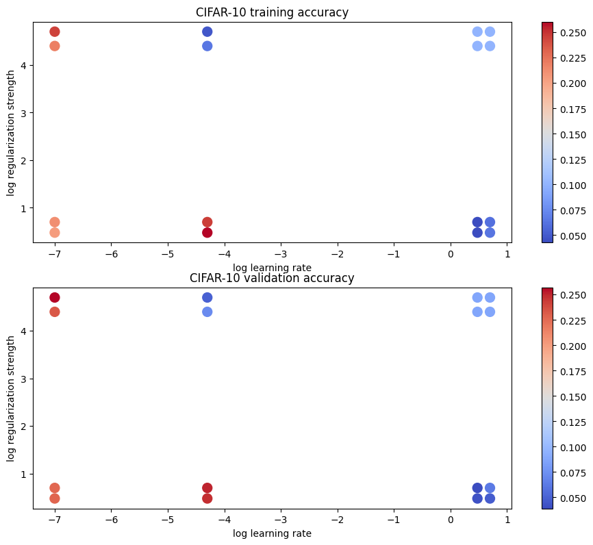
| # Visualize the cross-validation results
import math
import pdb
# pdb.set_trace()
x_scatter = [math.log10(x[0]) for x in results]
y_scatter = [math.log10(x[1]) for x in results]
# plot training accuracy
marker_size = 100
colors = [results[x][0] for x in results]
plt.subplot(2, 1, 1)
plt.tight_layout(pad=3)
plt.scatter(x_scatter, y_scatter, marker_size, c=colors, cmap=plt.cm.coolwarm)
plt.colorbar()
plt.xlabel('log learning rate')
plt.ylabel('log regularization strength')
plt.title('CIFAR-10 training accuracy')
# plot validation accuracy
colors = [results[x][1] for x in results] # default size of markers is 20
plt.subplot(2, 1, 2)
plt.scatter(x_scatter, y_scatter, marker_size, c=colors, cmap=plt.cm.coolwarm)
plt.colorbar()
plt.xlabel('log learning rate')
plt.ylabel('log regularization strength')
plt.title('CIFAR-10 validation accuracy')
plt.show()
|
1
2
3
4
| # Evaluate the best svm on test set
y_test_pred = best_svm.predict(X_test)
test_accuracy = np.mean(y_test == y_test_pred)
print('linear SVM on raw pixels final test set accuracy: %f' % test_accuracy)
|
1
| linear SVM on raw pixels final test set accuracy: 0.272000
|
1
2
3
4
5
6
7
8
9
10
11
12
13
14
15
| # Visualize the learned weights for each class.
# Depending on your choice of learning rate and regularization strength, these may
# or may not be nice to look at.
w = best_svm.W[:-1,:] # strip out the bias
w = w.reshape(32, 32, 3, 10)
w_min, w_max = np.min(w), np.max(w)
classes = ['plane', 'car', 'bird', 'cat', 'deer', 'dog', 'frog', 'horse', 'ship', 'truck']
for i in range(10):
plt.subplot(2, 5, i + 1)
# Rescale the weights to be between 0 and 255
wimg = 255.0 * (w[:, :, :, i].squeeze() - w_min) / (w_max - w_min)
plt.imshow(wimg.astype('uint8'))
plt.axis('off')
plt.title(classes[i])
|
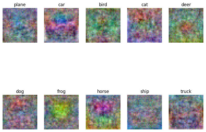
Inline question 2
Describe what your visualized SVM weights look like, and offer a brief explanation for why they look the way they do.
$\color{blue}{\textit Your Answer:}$
- 선형 SVM은 픽셀 간의 공간적 구조를 고려하지 않음
- RGB 채널 간 간섭
- 복잡한 데이터를 선형으로 분리하기 어려움
선형 SVM이 픽셀 단위로만 학습하기 때문에 노이즈에 가깝게 출력된다. SVM은 다른 특성은 배제하고 클래스 간 구분을 위한 가중치 텐서를 학습하기 때문에 시각적으로 해석하기 어려운 무작위에 가까운 패턴으로 보이게 된다.
